About the project
The Music Lights project is a system for visualising audio in a way that is hopefully fun and gives you a greater appreciation for how complex your music really is.
The project began as a small programming exercise originally born out of my desire to learn more about digital filters and to build an application for them in the real world. As I worked on the system sporadically in my free time, it started to evolve into a project worthy of a write-up and, in the end, I learned quite a lot about music theory, Fourier transformations, and digital filters. It was inspired by art installations such as Project Blinkenlights and this Heathrow Airport installation demoed by Mike Harrison. I liked the idea of a piece of electronic art that could transmute information from one of our senses to another.
Music Lights aims to represent the frequency content of your music in hues of red, green, and blue light; the music’s intensity is represented by the intensities of these colours.
This report outlines some of the theory behind the project in the fields of signal processing, and pure mathematics. It is published in parts as I write them, so follow along or jump to a part you find interesting!
Sampling theory
Music, like any audio, is an analogue, continuous, time-varying signal, which in this case, takes the form of reverberations in the air. In this analogue representation of sound, the behaviour of the air, speaker, or eardrum is well-defined at any arbitrary point in time. There is infinite precision in a continuous signal. This would be ideal for the perfect reproduction of music from a sound file or CD; the problem is there cannot exist a device or medium capable of containing the infinite amount of information it would take to encode an infinitely precise signal. Instead, what we can do is record a discretised, finite, digital representation of the original sound that will allow us to store and transmit the data and later re-create the original to some degree of accuracy. This digital representation can be created such that a perfect fidelity reconstruction is possible in which case the recording is said to be “lossless”. It can also sacrifice perfect fidelity and introduce an arbitrary degree of error, i.e., become “lossy”, in exchange for better performance in another metric such as file size. The following discussion presumes a lossless representation is desired.
On digital systems like computers, MP3 players, and CDs, one common method for storing audio is called “(Linear) Pulse-code Modulation” or PCM for short. In PCM, the amplitude of the signal is sampled at regular intervals and the amplitude value is quantised to the nearest integer value. The idea that a discretised version of a continuous signal can capture all of its information is known as the Nyquist-Shannon sampling theorem. Two important parameters of PCM are the sampling frequency and the bit depth. The first is simply the rate at which the original signal is sampled and quantised; the most important point here is that the highest frequency component which can later be perfectly reconstructed is limited to one-half of the sampling frequency. Stated precisely, the band-limit of the signal is up to, but not including, half of the sampling frequency. This is known as the Nyquist Criterion.
f_s>2B
Since the human ear is sensitive up to about 22 kHz in most healthy individuals, the most common music sampling frequencies are 44.1 kHz or 48 kHz. The second parameter, bit depth, is how many bits are used per sample to encode the amplitude. The more bits per sample, the smaller the difference in amplitude between any two adjacent values, and the more space required to store the samples. A 16-bit signed integer PCM is common in WAV files for example; there are 64536 levels of amplitude, 32 767 down to -32 768. In the real world, digital media files are reconstructed through a process known as “zero-order hold” not into their perfect analogue ancestors, but into quantised approximations as illustrated later.
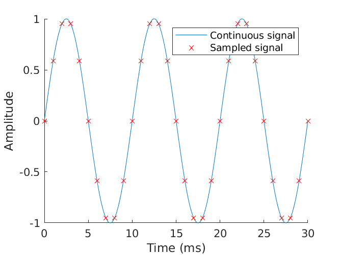
Above you can see a 100 Hz continuous-time signal in blue being sampled ten times per period, or at 1000 Hz. That is to say, the sampling frequency is 10 times the signal frequency, thus more than satisfying the Nyquist criterion. Because of this, it should be easy to see that given only the samples, and the assumption that the original was a sinusoid, you can only arrive at the one recreation of the original signal. If we really wanted to be frugal with our valuable bits and bytes, we could further reduce the sampling frequency to produce fewer samples while still capturing the original perfectly. The lowest sampling frequency that can accomplish this is called the “critical sampling frequency.”
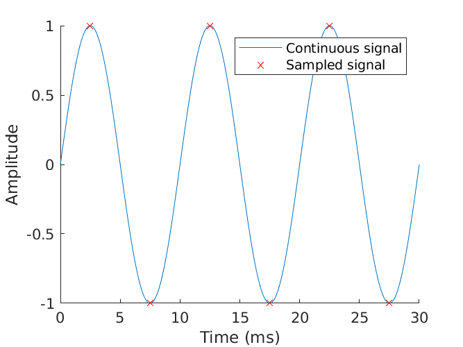
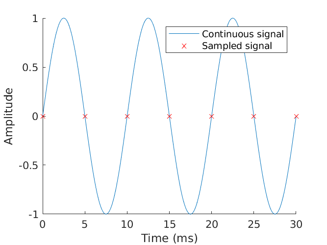
You can see the newly discretised representation only takes about one-sixth the number of samples as previously shown, but still produces the same result. Reducing the sampling rate any further would result in the scenario where the same samples could represent more than one signal. If multiple, different recreations can be represented by the same samples, the situation is ambiguous. These multiple signals would be aliases of each other. Aliasing is often unavoidable when sampling slower than the Nyquist frequency, and in the real world you would typically over-sample at some multiple of this rate so as to ensure you have enough data to later recreate the original, even in the case of minor imperfections during recording. For example, in this degenerate case, even sampling at the critical Nyquist frequency (and not strictly greater than it, as required by the Nyquist criterion) can yield an ambiguous situation. Here, the phase and frequency are well-defined, but any possible sinusoid amplitude fits the samples!
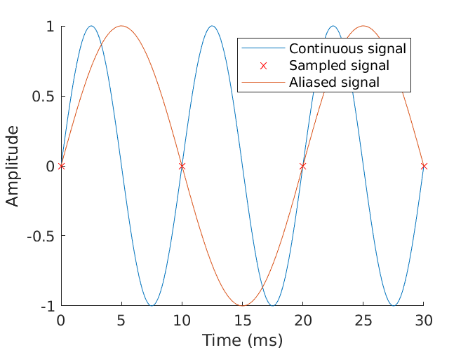
And finally, much worse, sampling below the Nyquist rate ensures we will misrepresent the data and draw the wrong conclusion from it. In this case, sampling only once per period, the data is reconstructed into a signal with half the frequency as the original. The original has been completely lost.
What these ideas tell us about our final system is that, simply, we need to sample the music at a rate at least twice as high as the highest frequency component of the sound we wish to capture or recreate. Whether it is implemented in hardware with an ADC sampling an audio line or sampled directly from digital media, the Nyquist criterion must be respected.
One last point is that in real-world systems, the sampled data isn’t reconstructed back into a perfect analogue representation, instead, the most common technique is to simply hold the amplitude of the signal at whatever the previous sample value was until the next is reached. This is called “zero-order hold” (ZOH) and works quite well if the sampling rate and bit depth are both sufficiently high. The following graphic displays the case where bit depth is indeed sufficiently high; since the original amplitude fits inside the sampling range, there is minimal quantisation error. However, the sampling rate is low enough that the reconstruction no longer closely resembles the original in shape. In the limit as both sampling frequency and bit depth approach infinity, the ZOH representation approaches perfect fidelity. If the values are sufficiently high, we aren’t able to perceive the small errors and the signal is perfect for all (human) intents and purposes.
x_{ZOH}(t) = \sum_{n=-\infty}^{\infty} x[n] \cdot \text{rect}(t - T/2 - nT)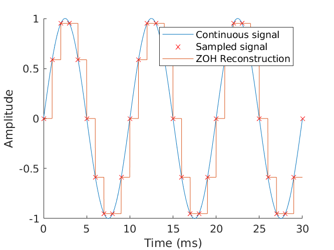
Fourier series and transform
So far, we’ve talked about “frequency components” of the sound being captured and reconstructed. But what is meant by this? In 1822 the French mathematician Jean-Baptiste Joseph Fourier examined how periodic signals could be broken down into a, potentially infinite, series of sinusoids each with its own amplitude and phase at some integer-multiple of the fundamental frequency. Creating an arbitrary, periodic waveform from base sinusoids is the synthesis of that signal. Going the opposite direction would be decomposing the combined signal into those base sinusoids. The Fourier series is a way to represent a periodic function as this sum of sinusoids. In other words, any periodic signal like a square wave, for example, is made up of sinusoids and can be decomposed back into a sum of those sinusoids. Using this square wave as an example, it is made up of a sinusoid of the fundamental frequency at unit amplitude, plus the summation of all odd multiples of this base frequency and at a scaled down amplitude.
x(t) = \sum_{n=0}^{\infty} \frac{1}{2n+1} \sin(2\pi \cdot 100\text{Hz} \cdot (2n+1))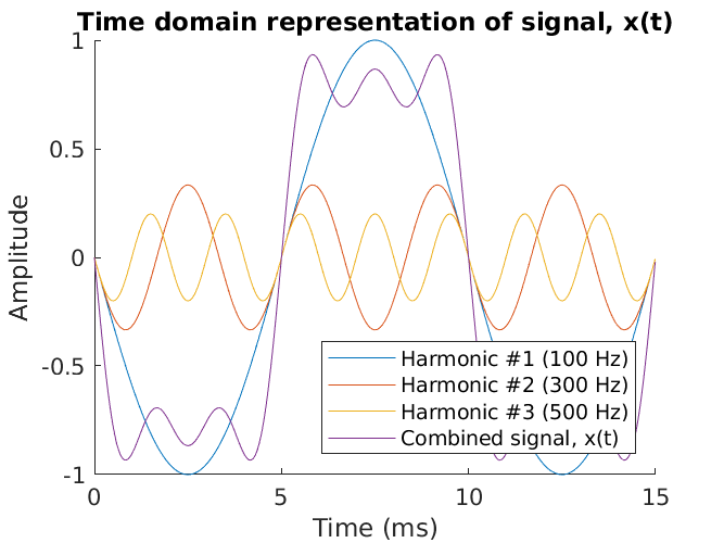
This plot looks complicated until it is broken down. The fundamental frequency component of 100 Hz is shown as the blue sinusoid and is also called the “first harmonic” of the signal. There are also two more harmonics which in this case are the first two odd multiples of 100 Hz, namely 300 Hz and 500 Hz. These are the third and fifth harmonics of the fundamental frequency. These sinusoidal harmonics are inversely scaled by their harmonic number so that they are one-third and one-fifth the amplitude of the fundamental respectively. If you were to sum up all three harmonics, it would yield the purple composite signal. You can see, with only three sinusoids in the series, the square wave already begins to take shape. Adding more harmonic sinusoids into the series continually improves the composite signal, approaching a perfect representation of the square wave at the limit of infinitely many harmonics. In reality, only a dozen or so harmonics would be required to yield a representation with an acceptably low error.
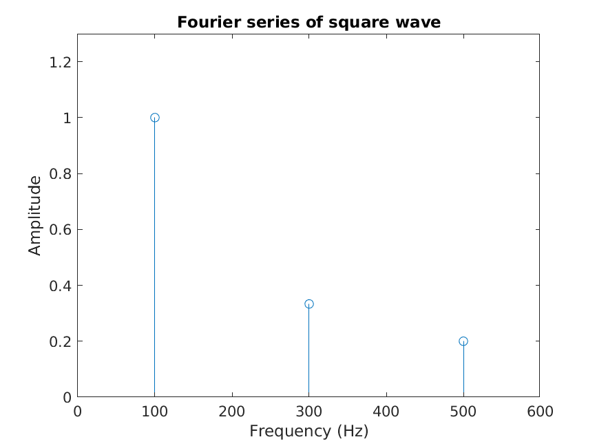
The three harmonics in the above time-domain signal can also be represented in an amplitude stem diagram of the Fourier series. Each stem encodes “how much” of each frequency makes up the original. Here, the three blue stems encode the purple, quasi-square wave above.
Expanding on this idea is the Fourier transform (FT). The Fourier transform has the nice benefit of being valid for more than periodic signals; any non-periodic “chunk” of a signal can be considered one period of some quasi-periodic signal made up of repeating the chunk. A signal represented as amplitude-vs-time is said to be in the time-domain whereas if it is decomposed via a Fourier method, you are considering the same signal in the frequency-domain. In this way, the FT is used to transform signals between these two domains, even non-periodic ones. One important distinction is whether the signals you are considering are made up of a continuous function in time, so called continuous-time signals, or are discretised representations, so called discrete-time signals. There are forward and reverse Fourier transformations for both cases, the continuous-time Fourier transformation (CTFT, or CFT), and the discrete-time Fourier transformation (DTFT, or DFT). One last complicated noodle in this alphabet soup is the Fast Fourier Transform (FFT), a specific algorithm for calculating the DFT faster than the rote definition of the transform on typical processor architectures. The FFT reduces the complexity of the DFT from O(n2) to O(n log n).
If we take the previous, purple, composite signal x(t) of three harmonics, and perform the DFT on it (since it is comprised of samples stored in an array on the computer), we can see what and how much of each frequency make it up.
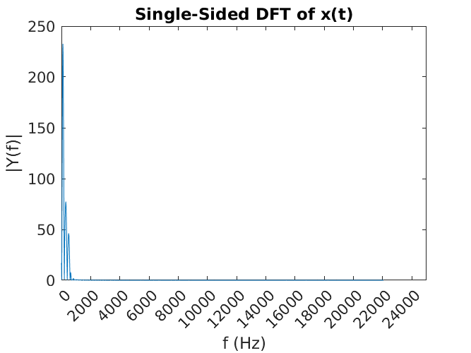
Well, that’s not much to look at. This plot displays all of the frequency content in the human audible range, all the way up to 22 050 Hz which was the sampling frequency. We know, however, that all the action (and energy of the signal) resides down in the hundreds of hertz. Zooming in on this region sheds a little more light on the make-up of that original signal.
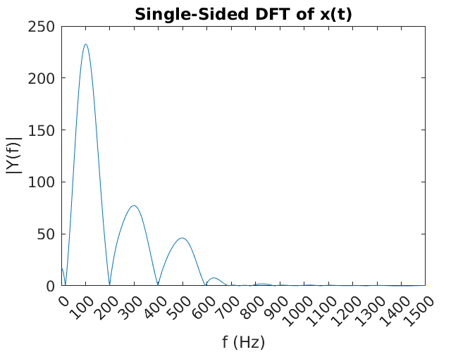
Now it is quite obvious that there is quite a bit of energy down at 100 HZ, the fundamental frequency, but also smaller components at 300 Hz and 500 Hz; about one third, and one fifth respectively. The Fourier transform has allowed us to break down the complicated periodic signal x(t) into a representation that shows its frequency-domain make up! In this way, we know the “recipe” of the original signal is a whole lot of 100 Hz sine wave, with a few dashes of 300 Hz, and a pinch of 500 Hz.
Compare the Fourier transform plot to the series plot above. See that they are very similar. The Fourier transform plot gives the impression that there is energy content at frequencies between 100 Hz and 300 Hz, 300 Hz and 500 Hz, and elsewhere when in fact there isn’t. This is a byproduct of the trade-off between sampling frequency and accuracy in the Fourier transform.
This transform is a ubiquitous tool of analysis in science, engineering and mathematics. It allows investigation into very complicated phenomena that evolve over time and/or space. It is difficult to overstate how ubiquitous the Fourier transform is in the STEM fields and even beyond. It is used to pick apart population data in censuses and animal populations, find patterns in financial trade data, find optimal geometries for grand theatres, and more.
Parseval’s Theorem
One detour worth talking about is Parseval’s theorem. Due to the unitary property of the Fourier transformation, the following identity holds:
\int_{-\infty}^{\infty} |x(t)|^2 \; dt = \int_{-\infty}^{\infty} |X(2\pi f)|^2 \; dfThis is to say, Parseval’s theorem gives the relationship between the integration of the squared function in time with the integration of the squared spectrum in frequency. Respectively, they yield the total energy of a signal by summing power-per-sample across time, or spectral power over frequency. Using Parseval’s theorem was actually a valid, tested solution to the whole project and resulted in a very concise program with the help of the NumPy. However, one purpose of the Music Lights project was to learn about digital filtering, hence we move forward to the next section!
Filtering
In the context of the Music Lights project, I was interested in extracting the relative magnitudes of three frequency ranges in the audio stream. In other words, I wanted to create a system that could make a distinction between the bass, mid-tones, and high pitch components of music and make decisions based on the amount of energy in each band. In this way, red lights could strobe away to the bass line of a song, while green would represent the typical vocal range of the artist while blue would flash with the strike of the high-hat.